Machine Learning Week 2
學習算法
- 多變量線性回歸
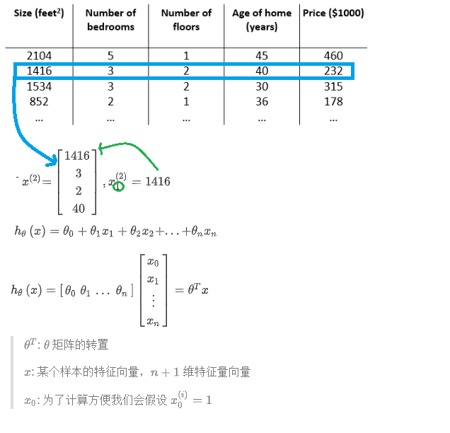
- 多特徵
- 多變量梯度下降
- 實踐
- 特徵值縮放
- 學習速率
- 如何確定函數是否收斂
- 多次迭代收斂法
- 無法確定需多少次迭代
- 比較容易畫迭代次數圖像
- 根據圖像易預測所需迭代次數
- 自動化測試收斂法(比較閥值)
- 閥值不易選
- 代價函數近乎直線時無法確定收斂
- 多次迭代收斂法
- 如何確定函數是否收斂
- 實踐
- 多特徵
- Octave 教學
- 下載安裝Octave
- 如何加載數據
pwd cd desktop ls load('featuresX.dat') load('priceY.dat') who %list all variables size(features) size(priceY) whos %detail variables clear features %delete a variable - 檔案features.dat內容
2104 3 1600 3 2400 3 3000 4 1985 4 1534 4 1427 3 1380 3 1494 3 1940 4 2000 3 1890 3 - 如何儲存數據
V=priceY(1:10) save hello.mat V clear %清除所有變數 save hello.txt v -ascii - 語法特性
- 分號的意思就是換到下一行
- 索引從1開始
- 函數怎麼用 help find
- A*B %A,B兩矩陣相乘
- A.*B %A,B兩矩陣內的每個元素做乘法運算,注意兩矩陣的大小要一樣

- 操作數據方法
A=[1 2;3 4;5 6] A(3,2) A(2,:) A(:,2) A([1 3],:) A(:,2)=[10;11;12] A=[A,[100,101,102]] A=[A,[100;101;102]] A(:) A=[1 2;3 4;5 6] B=[11 12;13 14;15 16] C=[A B]% 與[A,B]相同 C=[A;B] C=[1 1;2 2] A.^2 %平方 A*B %矩陣相乘 1./A %得到每個元素的倒數 log(A) exp(A) abs(A) -A A+1 A' A'' - 更多操作
  a=[1 15 2 0.5]
  max(a)
  [val,ind]=max(a)
  a<3
  find(a<3) %找a<3之索引
  A=magic(3) %行列對角加起來都是相同值
  >> A=magic(3)
  A =

     8   1   6
     3   5   7
     4   9   2

  >> [r,c]=find(A>=7)
  r =

     1
     3
     2

  c =

     1
     2
     3
  >> a=[1.0 15.0 2 0.5]
  a =

      1.00000   15.00000    2.00000    0.50000

  >> sum(a)
  ans =  18.500
  >> prod(a)
  ans =  15
  >> floor(a)
  ans =

      1   15    2    0

  >> ceil(a)
  ans =

      1   15    2    1
  >> max(A,[],1) %得到最大值,同max(A)
  ans =

     8   9   7
  >> max(A,[],2)
  ans =

     8
     7
     9

  >> A
  A =

     8   1   6
     3   5   7
     4   9   2
  >> max(max(A)) %找出整個矩陣的最大值
  ans =  9
  >> A=magic(9)
  >> sum(A,1)
  >> sum(A,2)
  >> sum(sum(A.*eye(9)))
  ans =  369
- 繪製數據
- 畫sin圖
t=[0:0.01:0.98]; y1=sin(2*pi*4*t); plot(t,y1) - 畫cos圖
y2=cos(2*pi*4*t); plot(t,y2) - 兩個圖重疊
  plot(t,y1)
  hold on
  plot(t,y2,'r')
  xlabel('time')
  ylabel('value')
  legend('sin','cos')
  title('myplot')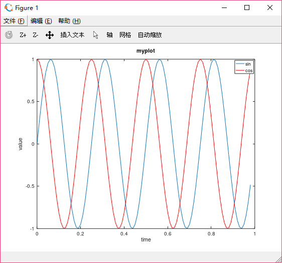
>> print –dpng 'myplot.png' %存圖 >> delete 'myplot.png' %刪圖 % 圖像標號 figure(1); plot(t, y1); figure(2); plot(t, y2); % 子圖 subplot(1,2,1) plot(t,y1) subplot(1,2,2) plot(t,y2) >> axis([0.5 1 0.6 1]) clf % 清除圖像 - 數值圖像表示
  >> imagesc(magic(15)),colorbar,colormap gray %用,連接可同時執行
  >> a=1,b=2,c=3
  a =  1
  b =  2
  c =  3
  >> a=1;b=2;c=3;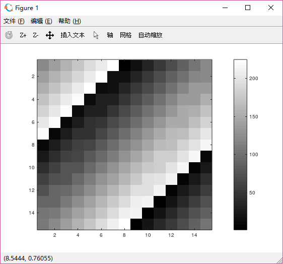
- 畫sin圖